Contents

% LR1_SVD_study.m
%
% A study in singular-value decomposition (SVD) in service of prediction.
% What matrix should be used to convert the raw scores of new cases that
% have not been part of the original SVD call?
%
%  File: work/RelExper/LRaven1/matlab/etc/LR1_SVD_study.m
%  Usage: publish('LR1_SVD_study.m','html') ;    % 'latex','doc','ppt'
%
% Reference: Great tutorial on PCA and SVD available on-line:
%  Shlens, J. (2009)  A Tutorial on Principal Component Analysis.
%  http://www.snl.salk.edu/~shlens/
%
% (c) Laboratory for Cognitive Modeling and Computational Cognitive
% Neuroscience at the Ohio State University, http://cogmod.osu.edu
%
% 1.0.2 2011-01-25 AAP: Scatterplot in Sect.280. LR1_R2_goalfun returns cvRMSE
%                       Ignore M_35x100_std when visualizing W in Sect.270.
% 1.0.1 2011-01-15 AAP: Swap var_idx and case_idx args to regress_subset
%                       Added cross-validation section 320
%                       Test cross-LRaven1_R2_goalfun.m in section 350
% 1.0.0 2011-01-14 AAP: Initial version, based on LRaven1_successor_plot.m

010: Get some data. In this script, we use data from LRaven1 experiment.

cd(fullfile(LRaven1_pathstr,'etc')) ;
fprintf('\n\nLR1_SVD_study executed on %s.\n\n',datestr(now)) ;
fprintf('cd %s\n',pwd) ;

clear all ; close all ;

LR1_SVD_study executed on 25-Jan-2011 19:17:11.

cd /Users/apetrov/a/r/w/work/RelExper/LRaven1/matlab/etc

020: Load H and the sequence data

% Load H
filename = fullfile(LRaven1_pathstr,'data','H.mat') ;
load(filename) ;

% Load temporal bin sequence data
trans_pathstr = fullfile(LRaven1_pathstr,'data','transitions') ;
filename = fullfile(trans_pathstr,'final_sequence.mat') ;
load(filename) ;

clearvars -except params H recoded_sequences

030: Define constants

params.gamma = 0.3 ;
params.lambda_gamma = 0.2 ;
params.lrate = 0.1 ;

% AOI and component number
N_AOIs = 10 ;                        % Areas of Interest (AOIs)
Tick=1:N_AOIs;
TickLabel='1|2|3|4|5|6|7|8|9|R';         % Interpretation of the 10 AOIs

NC = 3 ;         % Number of "best" components used in final regression
max_NC = 12 ;    % Max number of components, from which NC "best" are selected

TOL = 1e-8 ;   % tolerance for equality assertions

040: Define score targets based on cond and session info

% Slice these main score sets to get other options
omni_score_both = [H.session1_score]' + [H.session2_score]' ;   % [N_sbj 1]
omni_score_s1 = [H.session1_score]' ;
omni_score_s2 = [H.session2_score]' ;

050: Define Constants that vary based on cond and session

N_sbj = size(recoded_sequences,1) ;               % number of subjects
assert(size(recoded_sequences,1)==N_sbj) ;

N_trials = size(recoded_sequences,2) ;            % number of trials
assert(size(recoded_sequences,2)==N_trials) ;

060: Calculate successor rep for each sequence, with default params

M_by_sbj_by_trial = NaN([N_sbj,N_trials, N_AOIs N_AOIs]) ;
for s = 1:N_sbj
    for k = 1:N_trials

        %- isolate the sequence
        seq = recoded_sequences{s,k} ;

        %- Calculate and store the successor representation
        %  (If length(seq)==1, the result is a matrix of zeros.)
        M_by_sbj_by_trial(s,k,:,:) = successrep_learn(seq,N_AOIs,params) ;

        %-- Debug:
%         if (any(isnan(M(:))))
%             fprintf('s=%2d, k=%2d, gamma=%.6f, lrate=%.6f, l_g=%.6f returns NaN(s)\n',...
%                       s, k, params.gamma, params.lrate, params.lambda_gamma) ;
%         end
    end
end

clearvars s k seq

070: Average the SR matrices across trials:

M_by_sbj = squeeze(mean(M_by_sbj_by_trial,2)) ;  % [N_sbj N_AOIs N_AOIs]

080: Convert the 10x10 matrix to 1x100 row vector

N_vars = N_AOIs*N_AOIs ;
M_35x100 = reshape(M_by_sbj,N_sbj,N_vars) ;

090: Center the mean of each SR cell across Ss

[zM_35x100,M_35x100_mean,M_35x100_std] = zscore(M_35x100) ;

M_35x100_mean = mean(M_35x100) ;   % [1 x N_vars]
zM_35x100 = bsxfun(@minus,M_35x100,M_35x100_mean) ;    % zero mean

095: Does it help to divide by the std.deviation of each cell?

%divide_std_dev_p = false ;   % not recommended, see Sect.270
divide_std_dev_p = true ;   % recommended because yields more interpretable weights

if (divide_std_dev_p)
    M_35x100_std = std(M_35x100) ;     % [1 x N_vars]
    zM_35x100 = bsxfun(@rdivide,zM_35x100,M_35x100_std) ;  % unit std.dev
%else leave zM_35x100 alone
end


% zM_35x100 is the raw data matrix [N_subjects, N_vars] as far as SVD is concerned.

100: Principal Component Analysis using Shlens' conventions

% Compute components using SVD
% Numerically, PCA is an SVD of a centered data matrix
%
% In Shlens' tutorial, this is referred to as the "second method" described
% in Section VI and implemented in Matlab function pca2.m in Appendix B.

%- Step 0: Convert our matrix zM_35x100 to Shlens' conventions:
%   * rows = "dimensions" = variables in our terminology  % N_vars = 100
%   * columns = "cases" = subjects in our terminology     % N_sbj = 35
data = zM_35x100' ;    % [N_vars, N_sbj]
assert(size(data,1)==N_vars) ;
assert(size(data,2)==N_sbj) ;

%- Step 1: Centering -- already done for zM_35x100 in Section 090 above

%- Step 2: Construct the matrix Y
%  Note that data is transposed again and thus size(Y)==size(zM_35x100)
Y = data' ./ sqrt(N_sbj-1) ;  % Equation on top of page 9, left column

%- Step 3: Call SVD to decompose Y:  Y==U*Sigma*PC'
%  Full mode (as opposed to economical mode)
[U,Sigma,PC] = svd(Y) ;

%- Verify the identity that defines SVD:  Y == U*Sigma*PC'
Y_hat = U*Sigma*PC' ;
assert(max(abs(Y(:)-Y_hat(:)))<TOL) ;
clearvars Y_hat

%- Step 4: Calculate the variance for each PC
%  Note that var_PC(end)==0 (within rounding error) because we lost one
%  degree of freedom in the centering in Step 1 above.
var_PC = diag(Sigma).^2 ;       % [N_vars x 1]
assert(abs(var_PC(end))<TOL) ;

%- Step 5: Project the original data onto the orthogonal coordinate axes
%  defined by the principal components.  The result is a matrix of
%  "signals" of the same dimension as the input data matrix:
%   * rows = "dimensions" = variables in our terminology  % N_vars = 100
%   * columns = "cases" = subjects in our terminology     % N_sbj = 35
signals = PC' * data ;
assert(all(size(signals)==size(data))) ;

% Note that the bottom rows (N_sbj:N_vars) are zeros (within rounding err).
% This assumes that N_sbj<N_vars. Not sure what happens when N_sbj>N_vars.
foo = signals(N_sbj:N_vars,:) ;
assert(max(abs(foo(:)))<TOL) ;
clearvars foo

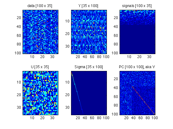
110: Plot a tableau of all matrices involved

Compare with Fig.4 in ShlensJ09.pdf

subplot(2,3,1) ;
foo = data ;
imagesc(abs(foo)) ;
title(sprintf('data [%d x %d]',size(foo,1),size(foo,2))) ;

subplot(2,3,2) ;
foo = Y ;
imagesc(abs(foo)) ;
title(sprintf('Y [%d x %d]',size(foo,1),size(foo,2))) ;

subplot(2,3,3) ;
foo = signals ;
imagesc(abs(foo)) ;
title(sprintf('signals [%d x %d]',size(foo,1),size(foo,2))) ;

subplot(2,3,4) ;
foo = U ;
imagesc(abs(foo)) ;
title(sprintf('U [%d x %d]',size(foo,1),size(foo,2))) ;

subplot(2,3,5) ;
foo = Sigma ;
imagesc(foo) ;
title(sprintf('Sigma [%d x %d]',size(foo,1),size(foo,2))) ;

subplot(2,3,6) ;
foo = PC ;
imagesc(abs(foo)) ;
title(sprintf('PC [%d x %d], aka V',size(foo,1),size(foo,2))) ;

clear foo

120: Archive these matrices and clear them from the workspace

full_mode_Shlens_layout.data = data ;
full_mode_Shlens_layout.Y = Y ;
full_mode_Shlens_layout.U = U ;
full_mode_Shlens_layout.Sigma = Sigma ;
full_mode_Shlens_layout.PC = PC ;
full_mode_Shlens_layout.signals = signals     %#ok<NOPTS>

clearvars data Y U Sigma PC signals

full_mode_Shlens_layout = 

       data: [100x35 double]
          Y: [35x100 double]
          U: [35x35 double]
      Sigma: [35x100 double]
         PC: [100x100 double]
    signals: [100x35 double]

130: Transpose the data so that variables (or "dimensions") are columns

Matlab's native format (and the format adopted for M_35x100) is:
 * rows = "cases" = subjects in our terminology           % N_sbj = 35
 * columns = "dimensions" = variables in our terminology  % N_vars = 100

Also, let's rename the variable "signals" to "projections".

Re-implement Shlens "second method", making the necessary transpositions:

%- Step 0: Our matrix zM_35x100 follows the Matlab convention:
%   * rows = "cases" = subjects in our terminology           % N_sbj = 35
%   * columns = "dimensions" = variables in our terminology  % N_vars = 100
data = zM_35x100 ;    % [N_sbj, N_vars]
assert(size(data,1)==N_sbj) ;
assert(size(data,2)==N_vars) ;

%- Step 1: Centering -- already done for zM_35x100 in Section 090 above
%  Note that Shens' algorithm used row-wise means:  mn=mean(data,2)
%  Thus, when we transpose data, we end up with the default column-wise
%  means which are implemented in the zscore call above

%- Step 2: Construct the matrix Y
%  Now we do *not* transpose. Thus size(Y)==size(zM_35x100) is still true:
Y = data ./ sqrt(N_sbj-1) ;  % Equation on top of page 9, left column

%- Step 3: Call SVD to decompose Y:  Y==U*Sigma*PC'
%  Full mode (as opposed to economical mode)
[U,Sigma,PC] = svd(Y) ;

%- Verify the identity that defines SVD:  Y == U*Sigma*PC'
Y_hat = U*Sigma*PC' ;
assert(max(abs(Y(:)-Y_hat(:)))<TOL) ;
clearvars Y_hat

%- Step 4: Calculate the variance for each PC
%  Note that var_PC(end)==0 (within rounding error) because we lost one
%  degree of freedom in the centering in Step 1 above.
var_PC = diag(Sigma).^2 ;       % [N_vars x 1]
assert(abs(var_PC(end))<TOL) ;

%- Step 5: Project the original data onto the orthogonal coordinate axes
%  defined by the principal components.  The result is a matrix of
%  "projections" of the same dimension as the input data matrix:
%   * rows = "cases" = subjects in our terminology           % N_sbj = 35
%   * columns = "dimensions" = variables in our terminology  % N_vars = 100
projections = data * PC ;
assert(all(size(projections)==size(data))) ;

% Now the rightmost columns (N_sbj:N_vars) are zeros (within rounding err).
% This assumes that N_sbj<N_vars. Not sure what happens when N_sbj>N_vars.
foo = projections(:,N_sbj:N_vars) ;   % [35x66]
assert(max(abs(foo(:)))<TOL) ;
clearvars foo

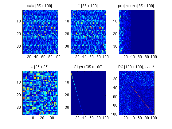
140: Plot a tableau of all matrices involved

Compare with Fig.4 in ShlensJ09.pdf

subplot(2,3,1) ;
foo = data ;
imagesc(abs(foo)) ;
title(sprintf('data [%d x %d]',size(foo,1),size(foo,2))) ;

subplot(2,3,2) ;
foo = Y ;
imagesc(abs(foo)) ;
title(sprintf('Y [%d x %d]',size(foo,1),size(foo,2))) ;

subplot(2,3,3) ;
foo = projections ;
imagesc(abs(foo)) ;
title(sprintf('projections [%d x %d]',size(foo,1),size(foo,2))) ;

subplot(2,3,4) ;
foo = U ;
imagesc(abs(foo)) ;
title(sprintf('U [%d x %d]',size(foo,1),size(foo,2))) ;

subplot(2,3,5) ;
foo = Sigma ;
imagesc(foo) ;
title(sprintf('Sigma [%d x %d]',size(foo,1),size(foo,2))) ;

subplot(2,3,6) ;
foo = PC ;
imagesc(abs(foo)) ;
title(sprintf('PC [%d x %d], aka V',size(foo,1),size(foo,2))) ;

clear foo

150: Archive these matrices and clear them from the workspace

full_mode.data = data ;
full_mode.Y = Y ;
full_mode.U = U ;
full_mode.Sigma = Sigma ;
full_mode.PC = PC ;
full_mode.projections = projections     %#ok<NOPTS>

clearvars data Y U Sigma PC projections

full_mode = 

           data: [35x100 double]
              Y: [35x100 double]
              U: [35x35 double]
          Sigma: [35x100 double]
             PC: [100x100 double]
    projections: [35x100 double]

160: Verify the equivalence

delta = full_mode.data - full_mode_Shlens_layout.data' ;   % transposed
assert(max(abs(delta(:)))<TOL) ;

delta = full_mode.PC - full_mode_Shlens_layout.PC ;    % NOT transposed
assert(max(abs(delta(:)))<TOL) ;

delta = full_mode.projections - full_mode_Shlens_layout.signals' ;  % transposed
assert(max(abs(delta(:)))<TOL) ;

clearvars delta

170: Run SVD in economy mode

We don't need more components than the rank of the data matrix (minus 1). Thus, there is no need for SVD to calculate their coefficients, given that the relevant entries in the Sigma matrix will be zeros. The code below has been tested assuming N_sbj < N_vars (35<100 in our case).

WARNING: Things may break when N_sbj >= N_vars. It is up to you to do the necessary tests (and, possibly, adjustments) if you need to analyze data with more cases than variables.

%- Step 0: Our matrix zM_35x100 follows the Matlab convention:
%   * rows = "cases" = subjects in our terminology           % N_sbj = 35
%   * columns = "dimensions" = variables in our terminology  % N_vars = 100
data = zM_35x100 ;    % [N_sbj, N_vars]
assert(size(data,1)==N_sbj) ;
assert(size(data,2)==N_vars) ;

%- Step 1: Centering -- already done for zM_35x100 in Section 090 above
%  Note that Shens' algorithm used row-wise means:  mn=mean(data,2)
%  Thus, when we transpose data, we end up with the default column-wise
%  means which are implemented in the zscore call above

%- Step 2: Construct the matrix Y
%  Now we do *not* transpose. Thus size(Y)==size(zM_35x100) is still true:
Y = data ./ sqrt(N_sbj-1) ;  % Equation on top of page 9, left column

%- Step 3: Call SVD to decompose Y:  Y==U*Sigma*PC'
%  ECONOMY mode (as opposed to full mode)
[U,Sigma,PC] = svd(Y,'econ') ;

% The identity that defines SVD still holds:  Y == U*Sigma*PC'
Y_hat = U*Sigma*PC' ;
assert(max(abs(Y(:)-Y_hat(:)))<TOL) ;
clearvars Y_hat

%- Step 4: Calculate the variance for each PC
%  Note that var_PC(end)==0 (within rounding error) because we lost one
%  degree of freedom in the centering in Step 1 above.
var_PC = diag(Sigma).^2 ;       % [N_vars x 1]
assert(abs(var_PC(end))<TOL) ;

% - Step 5: Project the original data onto the orthogonal coordinate axes
%  defined by the principal components.  The result is a matrix of
%  "projections" of the same dimension as the input data matrix:
%   * rows = "cases" = subjects in our terminology           % N_sbj = 35
%   * columns = "dimensions" = variables in our terminology  % truncated!
projections = data * PC ;     % [35 x 35] now rather than [35 x 100]

% It no longer holds that size(projections)==size(data)
% But the rightmost projections were useless anyway. We still have the
% low-numbered PCs, which are what we need for regressions and such.

180: Plot a tableau of all matrices involved

Compare with Fig.4 in ShlensJ09.pdf

subplot(2,3,1) ;
foo = data ;
imagesc(abs(foo)) ;
title(sprintf('data [%d x %d]',size(foo,1),size(foo,2))) ;

subplot(2,3,2) ;
foo = Y ;
imagesc(abs(foo)) ;
title(sprintf('Y [%d x %d]',size(foo,1),size(foo,2))) ;

subplot(2,3,3) ;
foo = projections ;
imagesc(abs(foo)) ;
title(sprintf('projections [%d x %d]',size(foo,1),size(foo,2))) ;

subplot(2,3,4) ;
foo = U ;
imagesc(abs(foo)) ;
title(sprintf('U [%d x %d]',size(foo,1),size(foo,2))) ;

subplot(2,3,5) ;
foo = Sigma ;
imagesc(foo) ;
title(sprintf('Sigma [%d x %d]',size(foo,1),size(foo,2))) ;

subplot(2,3,6) ;
foo = PC ;
imagesc(abs(foo)) ;
title(sprintf('PC [%d x %d], aka V',size(foo,1),size(foo,2))) ;

clear foo

190: Archive these matrices. Do not clear them from the workspace

econ_mode.data = data ;
econ_mode.Y = Y ;
econ_mode.U = U ;
econ_mode.Sigma = Sigma ;
econ_mode.PC = PC ;
econ_mode.projections = projections     %#ok<NOPTS>

econ_mode = 

           data: [35x100 double]
              Y: [35x100 double]
              U: [35x35 double]
          Sigma: [35x35 double]
             PC: [100x35 double]
    projections: [35x35 double]

200: Verify that economy mode returns a subset of what the full mode returns

Again, all this assumes that N_sbj<N_vars. It will not work otherwise.

delta = full_mode.U - econ_mode.U ;   % both are [N_sbj x N_sbj]
assert(max(abs(delta(:)))<TOL) ;

delta = full_mode.Sigma(:,1:N_sbj) - econ_mode.Sigma ;
assert(max(abs(delta(:)))<TOL) ;

delta = full_mode.PC(:,1:N_sbj) - econ_mode.PC ;
assert(max(abs(delta(:)))<TOL) ;

delta = full_mode.projections(:,1:N_sbj) - econ_mode.projections ;
assert(max(abs(delta(:)))<TOL) ;

clearvars delta

210: Multiple regression

Predict omni_score_both using the first max_NC projections

var_idx = (1:max_NC) ;
case_idx = (1:N_sbj)' ;   % do all subjects in this example, leave nobody out

reg12 = regress_subset(omni_score_both,projections,case_idx,var_idx) %#ok<NOPTS>

reg12 = 

           y: [35x1 double]
           X: [35x35 double]
     var_idx: [1 2 3 4 5 6 7 8 9 10 11 12]
    case_idx: [35x1 double]
          X1: [35x13 double]
        beta: [1x13 double]
          R2: 0.6150
        yhat: [35x1 double]

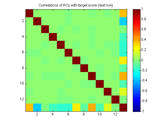
220: Correlate each component with the target score

The function utils/regression/select_components_Borda.m is based on this:

C = corrcoef([projections(:,var_idx) , omni_score_both]) ;  % [max_NC+1 x max_NC+1]

% Because the PCs form an orthonormal basis, the correlation matrix C is
% the identity matrix:
clf
imagesc(C,[-1 1]) ; axis square ; colorbar ;
title('Correlations of PCs with target score (last row)') ;


% The last row (and column) gives the correlation with the target score.
% As the PCs do not share variance, the *multiple* correlation R2 of a
% regression model using any subset of components simply equals the sum
% of the squared correlations with each individual component in the set
% and the target score:
diff_R2 = C(end,1:length(var_idx)).^2     %#ok<NOPTS>

calculated_R2 = sum(diff_R2(var_idx))     %#ok<NOPTS>
assert(max(abs(reg12.R2-calculated_R2))<TOL) ;

clearvars C calculated_R2

diff_R2 =

  Columns 1 through 11

    0.1402    0.1278    0.0000    0.0159    0.0268    0.0320    0.0773    0.0059    0.1495    0.0140    0.0256

  Column 12

    0.0000


calculated_R2 =

    0.6150

230: Select the top NC components with highest delta_R2

[ignore,idx] = sort(diff_R2,'descend') ;
best_comp = idx(1:NC)   %#ok<NOPTS>

best_comp =

     9     1     2

240: Re-run the regression on the best components

Note that this isn't really necessary -- the beta coefficients will be the same (again, because the PCs are orthogonal and don't share variance). Still, it is computationally cheap and implementaitonally easier just to re-run regress_subset on the best_comp index. It is also a safeguard against inconsistencies introduced by future changes in the code.

reg3 = regress_subset(omni_score_both,projections,case_idx,best_comp) %#ok<NOPTS>

calculated_R2 = sum(diff_R2(best_comp)) ;
assert(max(abs(reg3.R2-calculated_R2))<TOL) ;
clearvars calculated_R2

reg3 = 

           y: [35x1 double]
           X: [35x35 double]
     var_idx: [9 1 2]
    case_idx: [35x1 double]
          X1: [35x4 double]
        beta: [0.8171 0.3063 -0.3280 21.9429]
          R2: 0.4176
        yhat: [35x1 double]

250: Define a benchmark data set

Suppose a new subject comes in, one whose successor rep was not part of the SVD call that defined the components. We want to be able to predict the Raven score for such new subject(s). To that end, we stack all the linear transformations into a single weight vector and a single additive constant term.

To help wrap our heads around this, let's recapitulate the steps. We'll do it on new_M that just happens to be a random permutation of the original M.

old2new_mapping = randperm(N_sbj) ;
new_M = M_35x100(old2new_mapping,:) ;
benchmark_yhat = reg3.yhat(old2new_mapping) ;

260: Calculate weights that can predict scores for arbitrary data

We will work backwards, beginning with the last step and going up: 1. yhat = projections(:,best_comp) * beta(1:NC)' + beta(NC+1) 2. projections(:,best_comp) = data * PC(:,best_comp) ; 3. yhat = (data * PC(:,best_comp)) * beta(1:NC)' + beta(NC+1) 4. data = zscore(M) = (M-mean_M)./std_M 5. yhat = (((M-mean_M)./std_M) * PC(:,best_comp)) * beta(1:NC)' + beta(NC+1) 6. (M./s) * P = M * (P./s) 7. yhat = ((M-mean_M) * (PC(:,best_comp)./std_M)) * beta(1:NC)' + beta(NC+1) 8. Let Z:=(PC(:,best_comp)./std_M)) ; b:=beta(1:NC)' ; c1:=beta(NC+1) 9. yhat = (M-mean_M)*Z*b + c1

%10. yhat = M*Z*b - mean_M*Z*b + c1 = M*Z*b + (c1-mean_M*Z*b)
%11. Weights W = Z*b = (PC(:,best_comp)./std_M)) * beta(1:NC)'
%12. Alternatively: W = (PC(:,best_comp)*beta(1:NC)') ./std_M
%13. additive_const = beta(NC+1) - W*mean_M

% Calculate weight vector W [= weight_matrix(:)] defined in 12. above:
% Note that this combines the NC components into a single weight vector.
W = PC(:,best_comp) * reg3.beta(1:NC)' ;   % [N_vars x NC] * [NC x 1] = [N_vars x 1]

W1 = W ;    % for plotting in Sect. 270 below

if (divide_std_dev_p)
    W = W ./ M_35x100_std' ;
%else leave W alone
end

% Additive constant from step 12. above
const_term = reg3.beta(end) - M_35x100_mean * W     %#ok<NOPTS>

const_term =

   15.3969

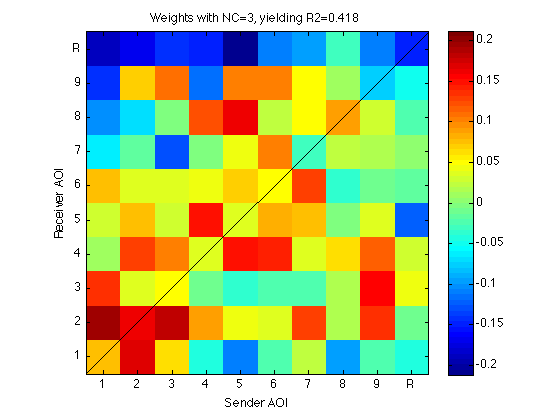
270: Visualize W1 as a matrix

clf
mmm = 0.8*max(abs(W1(:))) ;
imagesc(reshape(W1,N_AOIs,N_AOIs),[-mmm mmm]);
title(sprintf('Weights with NC=%d, yielding R2=%.3f',NC,reg3.R2)) ;

axis xy;axis square;colorbar ;
h=refline(1,0);set(h,'Color','k'); clear h
set(gca,'XTick',Tick,'XTickLabel',TickLabel,'YTick',Tick,'YTickLabel',TickLabel);
xlabel('Sender AOI'); ylabel('Receiver AOI');

clearvars mmm

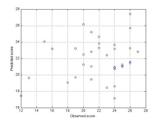
280: Predict benchmark scores using W

weight_based_yhat = new_M * W + const_term ;    % [size(new_M,1) x 1]

clf
plot(omni_score_both,weight_based_yhat,'o') ;
xlabel('Observed score') ;
ylabel('Predicted score') ;
grid on

290: Verify that weight_based_yhat == benchmark_yhat

discrepancy = weight_based_yhat - benchmark_yhat ;
describe(discrepancy)

assert(max(abs(discrepancy))<TOL) ;

    Mean  Std.dev       Min     Q25  Median     Q75     Max
------------------------------------------------------------
  -0.000    0.000     -0.00   -0.00    0.00    0.00    0.00

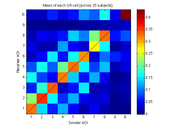
300: Visualize M_35x100_mean as a matrix

clf
mmm = 0.5*max(abs(M_35x100_mean(:))) ;
imagesc(reshape(M_35x100_mean,N_AOIs,N_AOIs),[0 mmm]);
title(sprintf('Mean of each SR cell (across %d subjects)',N_sbj)) ;

axis xy;axis square;colorbar ;
h=refline(1,0);set(h,'Color','k'); clear h
set(gca,'XTick',Tick,'XTickLabel',TickLabel,'YTick',Tick,'YTickLabel',TickLabel);
xlabel('Sender AOI'); ylabel('Receiver AOI');

clearvars mmm

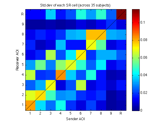
310: Visualize M_35x100_std as a matrix

if (divide_std_dev_p)
    clf
    mmm = 0.8*max(abs(M_35x100_std(:))) ;
    imagesc(reshape(M_35x100_std,N_AOIs,N_AOIs),[0 mmm]);
    title(sprintf('Std.dev of each SR cell (across %d subjects)',N_sbj)) ;

    axis xy;axis square;colorbar ;
    h=refline(1,0);set(h,'Color','k'); clear h
    set(gca,'XTick',Tick,'XTickLabel',TickLabel,'YTick',Tick,'YTickLabel',TickLabel);
    xlabel('Sender AOI'); ylabel('Receiver AOI');

    clearvars mmm
%else  do nothing: M_35x100_std is just a vector of 1s
end

320: Cross-validated R-square

Let's use (and test) the newly defined utils/regress/cross_validated_R2.m. We will do a leave-TWO-out cross validation, 595 (=35*34/2) sets in total.

N_left_out = 2 ;   % leave two cases (=subjects) from each set
case_sets = nchoosek(1:N_sbj,N_sbj-N_left_out) ;

cvR = cross_validated_R2(omni_score_both,projections,case_sets,best_comp) %#ok<NOPTS>
describe(cvR.R2_set)

cvR = 

             y: [35x1 double]
             X: [35x35 double]
     case_sets: [595x33 double]
          beta: [595x4 double]
        R2_set: [595x1 double]
       y_train: [595x33 double]
        y_test: [595x2 double]
    yhat_train: [595x33 double]
     yhat_test: [595x2 double]
      R2_train: 0.4230
       R2_test: 0.2427
    RMSE_train: 2.8067
     RMSE_test: 3.2769


    Mean  Std.dev       Min     Q25  Median     Q75     Max
------------------------------------------------------------
   0.421    0.037      0.29    0.41    0.42    0.44    0.54

330: Sanity check: Scramble the scores and cross-validate again

scramble_idx = randperm(N_sbj) ;

cvR_scrambled = cross_validated_R2(omni_score_both(scramble_idx),...
                                   projections,case_sets,best_comp) %#ok<NOPTS>
describe(cvR_scrambled.R2_set)

cvR_scrambled = 

             y: [35x1 double]
             X: [35x35 double]
     case_sets: [595x33 double]
          beta: [595x4 double]
        R2_set: [595x1 double]
       y_train: [595x33 double]
        y_test: [595x2 double]
    yhat_train: [595x33 double]
     yhat_test: [595x2 double]
      R2_train: 0.2245
       R2_test: 0.0473
    RMSE_train: 3.2540
     RMSE_test: 3.7166


    Mean  Std.dev       Min     Q25  Median     Q75     Max
------------------------------------------------------------
   0.224    0.048      0.09    0.20    0.22    0.24    0.44

340: Prepare to call LRaven1_R2_goalfun.m

This is a test of ../prog/LRaven1_R2_goalfun.m, which was developed on the basis of the current script.

%- Prepare the structure D, which holds the original fixation sequences
D.sequences = recoded_sequences ;
D.target = omni_score_both ;

%- Prepare search_params
search_params.N_AOIs = N_AOIs ;

search_params.N_comp = NC ;
search_params.max_N_comp = max_NC ;

search_params.sbj_idx = (1:N_sbj) ;      % that is, all subjects
search_params.trial_idx = (1:N_trials) ; % all trials

search_params.N_left_out = N_left_out ;
search_params.Borda_diagnosep = true   %#ok<NOPTS>

%- To avoid recalculating the SRs, add them to D:
D.SR_params = params ;
D.trial_idx = search_params.trial_idx ;
D.SR_by_sbj = M_35x100 %#ok<NOPTS>

search_params = 

             N_AOIs: 10
             N_comp: 3
         max_N_comp: 12
            sbj_idx: [1x35 double]
          trial_idx: [1 2 3 4 5 6 7 8 9 10 11 12 13 14 15 16 17 18 19 20 21 22 23 24 25 26 27 28]
         N_left_out: 2
    Borda_diagnosep: 1


D = 

    sequences: {35x28 cell}
       target: [35x1 double]
    SR_params: [1x1 struct]
    trial_idx: [1 2 3 4 5 6 7 8 9 10 11 12 13 14 15 16 17 18 19 20 21 22 23 24 25 26 27 28]
    SR_by_sbj: [35x100 double]

350: Verify that LRaven1_R2_goalfun reproduces the components

%- Call LRaven1_R2_goalfun
SR_params = [params.gamma params.lambda_gamma params.lrate] ;
%[cvR2,cvR2_train,export] = LRaven1_R2_goalfun(SR_params,D,search_params) %#ok<NOPTS>
[cvRMSE,export] = LRaven1_R2_goalfun(SR_params,D,search_params) %#ok<NOPTS>

%- Verify that it has indeed used the cached SRs
assert(~isfield(export,'SR_by_sbj_by_trial')) ;
assert(~isfield(export,'SR_by_sbj')) ;

if (divide_std_dev_p)
    %- Verify that it called SVD on the same DATA matrix
    assert(max(abs(export.data(:)-data(:)))<TOL) ;

    %- Verify that it got the same U, Sigma, and PC
    assert(max(abs(export.U(:)-U(:)))<TOL) ;
    assert(max(abs(export.PC(:)-PC(:)))<TOL) ;

    sigma = diag(Sigma) ;
    assert(max(abs(export.Sigma(:)-sigma(:)))<TOL) ;
    clearvars sigma

    %- Verify that it thereby arrived at the same projections
    assert(max(abs(export.projections(:)-projections(:)))<TOL) ;
end % if (~divide_std_dev_p)

cvRMSE =

    3.2769


export = 

         search_params: [1x1 struct]
             SR_params: [1x1 struct]
    mean_SR_across_sbj: [1x100 double]
     std_SR_across_sbj: [1x100 double]
                  data: [35x100 double]
                     U: [35x35 double]
                 Sigma: [35x1 double]
                    PC: [100x35 double]
           projections: [35x35 double]
          mean_R2_gain: [1x35 double]
         unanim_scores: [1.0417 0.9333 0.8417 0.7500 0.6667 0.5833 0.5000 0.4167 0.3333 0.2500 0.1667 0.0833]
        ordered_scores: [0.9483 0.9087 0.8686 0.7537 0.5825 0.5556 0.5237 0.4091 0.3864 0.2602 0.1584 0.1448]
              best_idx: [9 1 2 7 6 5 11 4 10 8 12 3]
      max_offdiag_corr: [595x1 double]
         Borda_winners: [9 1 2]
                R2_set: [595x1 double]
              R2_train: 0.4230
               R2_test: 0.2427
            RMSE_train: 2.8067
             RMSE_test: 3.2769

360: Are the Borda components the same as the globally selected ones?

LRaven1_R2_goalfun.m calls utils/regression/select_components_Borda.m which institutes an "election" of components across several hundred cross-validation sets (or "voters"). If all goes well, the election winners should match the best_comp above, although this is not a mathematical necessity. See http://en.wikipedia.org/wiki/Borda_count

Borda_winners = export.Borda_winners %#ok<NOPTS>

describe(export.max_offdiag_corr) ;

% For this data set, the assumption of (approximate) orthogonality holds up
% reasonably well -- the average off-diagonal correlations (~0.14) are
% unlikely to change the ranks of the R2_gain of the components.
% For smaller data sets (fewer subjects), however, the off-diagonal
% correlations have been observed to get as high as 0.7, which is a problem.


%- If Borda_winners==best_comp, the cross-validation results should match
if (all(Borda_winners==best_comp))
    if (~divide_std_dev_p)
        assert(max(abs(cvR.R2_set(:)-export.R2_set(:)))<TOL) ;
        assert(max(abs(cvR.R2_train-export.R2_train))<TOL) ;
        assert(max(abs(cvR.R2_test-export.R2_test))<TOL) ;
    end
else
    fprintf('Borda_winners %s different from global winners %s\n',...
        mat2str(Borda_winners), mat2str(best_comp)) ;
end

Borda_winners =

     9     1     2


    Mean  Std.dev       Min     Q25  Median     Q75     Max
------------------------------------------------------------
   0.138    0.047      0.04    0.11    0.13    0.16    0.32

999: Finish

close all

%%%%% End of file LR1_SVD_study.m

Published with MATLAB® 7.10